I Analyzed 6TB of Raw Stock Market Data to Uncover the 30 Most Consistently Traded Stocks — Here’s What I Found
What if you could replay the last 9 years of market activity — every quote, every trade — and figure out which stocks have never left the party?
 Last Friday, a quiet challenge came up in a conversation. Someone with a sharp mathematical mind and a preference for staying behind the scenes posed a deceptively simple question: "Which stocks have been traded the most, consistently, from 2016 to today?"
That one question sent me down a 27-hour rabbit hole…
Last Friday, a quiet challenge came up in a conversation. Someone with a sharp mathematical mind and a preference for staying behind the scenes posed a deceptively simple question: "Which stocks have been traded the most, consistently, from 2016 to today?"
That one question sent me down a 27-hour rabbit hole…
We had the data: 6TB of IEX tick captures spanning 2'187 PCAP files and over 22'119 unique symbols. We had the tools: an HDF5-backed firehose built for high-frequency analytics in pure C++23.
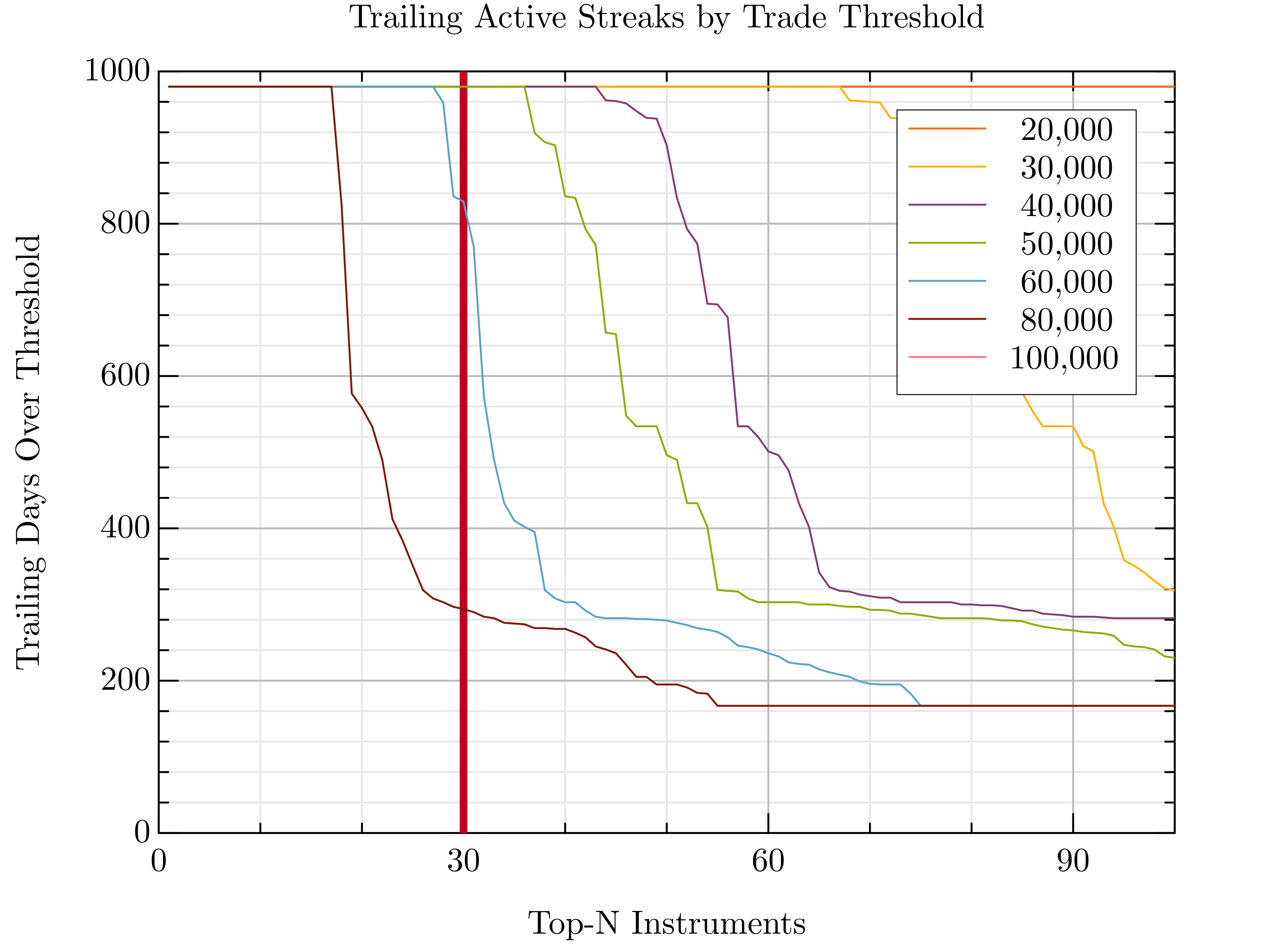
What followed was a misadventure in semantics. I first averaged trade counts across all dates — a rookie mistake. Turns out, averaging doesn’t guarantee consistency — some stocks burn bright for a while, then disappear. That oversight cost me half a day of CPU time and a good chunk of humility. The fix? A better idea: walk backwards from today and look for the longest uninterrupted streak of trading activity for each stock. Luckily, the 12 hours spent building the index weren’t wasted — that heavy lifting could be recycled for the new logic. Implementation time? 30 minutes. Execution time? 5 seconds. Victory? Priceless.
Here’s what we found.
Step 1 — Convert PCAPs into Stats with IEX2H5
Before we can rank stocks, we need summary statistics from the raw IEX market data feeds. That’s where iex2h5 comes in — a high-performance HDF5-based data converter purpose-built for handling PCAP dumps from IEX.
To extract stats only (and skip writing any tick data), we use the --command none mode. We'll name the output file something meaningful like statistics.h5, and pass in a file glob — the glorious Unix-era invention (from B at Bell Labs) — pointing to our compressed dataset, e.g. /lake/iex/tops/*.pcap.gz.
Of course, we’re all lazy, so let’s use the short forms -c, -o, and let iex2h5 do its thing:
steven@saturn:~/shared-tmp$ iex2h5 -c none -o statistics.h5 /lake/iex/tops/*.pcap.gz
[iex2h5] Converting 2194 files using backend: hdf5 — using 1 thread — © Varga Consulting, 2017–2025
[iex2h5] Visit https://vargaconsulting.github.io/iex2h5/ — Star it, Share it, Support Open Tools ⭐️
▫ 2016-12-13 14:30:00 21:00:00 ✓
▫ 2016-12-14 14:30:00 21:00:00 ✓
▫ 2016-12-15 17:31:52 21:00:00 ✓
[...]
▫ 2025-08-22 14:30:00 21:00:00 ✓
▫ 2025-08-25 14:30:00 21:00:00 ✓
▫ 2025-08-26 14:30:00 21:00:00 ✓
benchmark: 259159357724 events in 44087097ms  5.9 Mticks/s, 0.170000 µs/tick latency, 5758.33 GiB input converted into 733.97 MiB output
[iex2h5] Conversion complete — all files processed successfully
[iex2h5] Market data © IEX — Investors Exchange. Attribution required. See https://iextrading.com
What you get is a compact HDF5 file containing:
/instruments→ all unique stock symbols (22,119)/trading_days→ the full trading calendar (2,187 days)/stats→ per-symbol statistics across all days (e.g. trade volume, trade count, first/last seen)
On the performance side:
- Raw storage throughput (ZFS): ~254 MB/s
- End-to-end pipeline throughput: 5.76 TB of compressed PCAP input in 44,087 s → ~130 MB/s effective
- Event rate: ~5.9 million ticks/sec sustained
From here you’re ready to rank, filter, and extract the top performers. The best part? A full 6 TB dataset was processed in ~12 hours — on a single desktop workstation, using a single-threaded execution model. No cluster, no parallel jobs.
These results form a solid baseline: the upcoming commercial version will extend the engine to a multi-process, multi-threaded execution model, scaling performance well beyond what a single core can deliver.
Step 2 — digest the statistics
Top-K Trade Streak Filter for Julia
Top-K Trade Streak Filter for Python
HDF5 data dump h5dump topk.h5
Julia Plot
Step 3 — Reprocess the Tick Data for the Top 30 Stocks
Now that we’ve identified the most consistently active stocks, it’s time to zoom in and reprocess just the relevant PCAP files. If you already have tick-level HDF5 output, you’re set. But if not, here's a neat trick: use good old Unix GLOB patterns to cherry-pick just the days you need — no need to touch all 6TB again.
For example, let’s reconstruct a trading window around September 2021:
iex2h5 -c irts -o top30.h5 /lake/iex/tops/TOPS-2021-09-1{3,4,5,6,7,8,9}.pcap.gz  # fractional start
iex2h5 -c irts -o top30.h5 /lake/iex/tops/TOPS-2021-09-{2,3}?.pcap.gz            # rest of the month
And then stitch together additional months or years:
iex2h5 -c irts -o top30.h5 /lake/iex/tops/TOPS-2021-1{0,1,2}-??.pcap.gz
iex2h5 -c irts -o top30.h5 /lake/iex/tops/TOPS-202{2,3,4,5}-??-??.pcap.gz
These globs target specific slices of the timeline while keeping file-level parallelism open for future optimization. And of course, you can always batch them via xargs.
Top-K Trade Streak Filter for Julia
System Specs — Single Desktop Workstation (ZFS-backed)
This entire pipeline was executed on a single desktop workstation — no cluster, no GPU, no cloud — just efficient C++ and smart data layout:
- CPU: Intel Core i7‑11700K @ 3.60 GHz (8 cores / 16 threads)
- RAM: 64 GiB DDR4
- Scratch Disk: 3.6 TB NVMe SSD (
/mnt) - Main Archive: 15 TB ZFS pool (
/lake), spanned 2× 8 TB HDDs- Pool name:
lake, Dataset:lake/stock, Compression: off (default), Recordsize: 128K (default), Deduplication: off
- Pool name:
- 🐧 OS: Ubuntu 22.04 LTS
Read performance of ZFS based Lake 254MB/s sustained
steven@saturn:~$ sudo fio --name=zfs_seq_read_real --filename=/lake/fio-read-test.bin
    --rw=read --bs=1M --size=100G --numjobs=1 --ioengine=psync --direct=1 --group_reporting

zfs_seq_read_real: (g=0): rw=read, bs=(R) 1024KiB-1024KiB, (W) 1024KiB-1024KiB, (T) 1024KiB-1024KiB, ioengine=psync, iodepth=1
fio-3.28
Starting 1 process
zfs_seq_read_real: Laying out IO file (1 file / 102400MiB)
Jobs: 1 (f=1): [R(1)][100.0%][r=180MiB/s][r=180 IOPS][eta 00m:00s]
zfs_seq_read_real: (groupid=0, jobs=1): err= 0: pid=2897558: Sat Aug 30 16:40:16 2025
read: IOPS=242, BW=243MiB/s (254MB/s)(100GiB/422156msec)
    clat (usec): min=103, max=326105, avg=4118.30, stdev=8610.69
    lat (usec): min=104, max=326105, avg=4118.72, stdev=8610.67
    clat percentiles (usec):
    |  1.00th=[   208],  5.00th=[   229], 10.00th=[   277], 20.00th=[   824],
    | 30.00th=[   865], 40.00th=[   914], 50.00th=[  4146], 60.00th=[  4817],
    | 70.00th=[  5276], 80.00th=[  5800], 90.00th=[  6587], 95.00th=[  7767],
    | 99.00th=[ 33817], 99.50th=[ 61080], 99.90th=[102237], 99.95th=[139461],
    | 99.99th=[299893]
bw (  KiB/s): min=16384, max=395264, per=100.00%, avg=248505.24, stdev=59429.03, samples=843
iops        : min=   16, max=  386, avg=242.68, stdev=58.04, samples=843
lat (usec)   : 250=8.07%, 500=4.03%, 750=2.97%, 1000=28.82%
lat (msec)   : 2=1.16%, 4=3.06%, 10=49.77%, 20=0.87%, 50=0.56%
lat (msec)   : 100=0.60%, 250=0.08%, 500=0.03%
cpu          : usr=0.21%, sys=15.68%, ctx=58582, majf=0, minf=270
IO depths    : 1=100.0%, 2=0.0%, 4=0.0%, 8=0.0%, 16=0.0%, 32=0.0%, >=64=0.0%
    submit    : 0=0.0%, 4=100.0%, 8=0.0%, 16=0.0%, 32=0.0%, 64=0.0%, >=64=0.0%
    complete  : 0=0.0%, 4=100.0%, 8=0.0%, 16=0.0%, 32=0.0%, 64=0.0%, >=64=0.0%
    issued rwts: total=102400,0,0,0 short=0,0,0,0 dropped=0,0,0,0
    latency   : target=0, window=0, percentile=100.00%, depth=1

Run status group 0 (all jobs):
READ: bw=243MiB/s (254MB/s), 243MiB/s-243MiB/s (254MB/s-254MB/s), io=100GiB (107GB), run=422156-422156msec
Read performance of NVME scratch disk 4GB/s sustained
steven@saturn:~$ sudo fio --name=nvme_seq_read_real --filename=/home/steven/scratch/fio-read-test.bin
    --rw=read --bs=1M --size=100G --numjobs=1 --ioengine=psync --direct=1 --group_reporting
nvme_seq_read_real: (g=0): rw=read, bs=(R) 1024KiB-1024KiB, (W) 1024KiB-1024KiB, (T) 1024KiB-1024KiB, ioengine=psync, iodepth=1
fio-3.28
Starting 1 process
nvme_seq_read_real: Laying out IO file (1 file / 102400MiB)
Jobs: 1 (f=1): [R(1)][100.0%][r=3203MiB/s][r=3203 IOPS][eta 00m:00s]
nvme_seq_read_real: (groupid=0, jobs=1): err= 0: pid=3047825: Sat Aug 30 18:28:21 2025
read: IOPS=3847, BW=3848MiB/s (4035MB/s)(100GiB/26613msec)
    clat (usec): min=180, max=3871, avg=259.65, stdev=79.55
    lat (usec): min=180, max=3871, avg=259.68, stdev=79.56
    clat percentiles (usec):
    |  1.00th=[  198],  5.00th=[  200], 10.00th=[  202], 20.00th=[  202],
    | 30.00th=[  202], 40.00th=[  204], 50.00th=[  206], 60.00th=[  237],
    | 70.00th=[  310], 80.00th=[  318], 90.00th=[  371], 95.00th=[  400],
    | 99.00th=[  502], 99.50th=[  529], 99.90th=[  660], 99.95th=[  676],
    | 99.99th=[ 1106]
bw (  MiB/s): min= 2774, max= 4912, per=100.00%, avg=3852.79, stdev=798.23, samples=53
iops        : min= 2774, max= 4912, avg=3852.79, stdev=798.23, samples=53
lat (usec)   : 250=60.44%, 500=38.55%, 750=0.99%, 1000=0.01%
lat (msec)   : 2=0.01%, 4=0.01%
cpu          : usr=0.09%, sys=8.43%, ctx=102484, majf=0, minf=267
IO depths    : 1=100.0%, 2=0.0%, 4=0.0%, 8=0.0%, 16=0.0%, 32=0.0%, >=64=0.0%
    submit    : 0=0.0%, 4=100.0%, 8=0.0%, 16=0.0%, 32=0.0%, 64=0.0%, >=64=0.0%
    complete  : 0=0.0%, 4=100.0%, 8=0.0%, 16=0.0%, 32=0.0%, 64=0.0%, >=64=0.0%
    issued rwts: total=102400,0,0,0 short=0,0,0,0 dropped=0,0,0,0
    latency   : target=0, window=0, percentile=100.00%, depth=1

Run status group 0 (all jobs):
READ: bw=3848MiB/s (4035MB/s), 3848MiB/s-3848MiB/s (4035MB/s-4035MB/s), io=100GiB (107GB), run=26613-26613msec

Disk stats (read/write):
nvme0n1: ios=220152/422, merge=0/15, ticks=44398/64, in_queue=44537, util=99.70
Write performance of NVME scratch disk 2GB/s sustained
steven@saturn:~$ sudo fio --name=nvme_seq_write_real --filename=/home/steven/scratch/fio-write-test.bin
    --rw=write --bs=1M --size=100G --numjobs=1 --ioengine=psync --direct=1 --group_reporting

nvme_seq_write_real: (g=0): rw=write, bs=(R) 1024KiB-1024KiB, (W) 1024KiB-1024KiB, (T) 1024KiB-1024KiB, ioengine=psync, iodepth=1
fio-3.28
Starting 1 process
nvme_seq_write_real: Laying out IO file (1 file / 102400MiB)
Jobs: 1 (f=1): [W(1)][100.0%][w=1410MiB/s][w=1410 IOPS][eta 00m:00s]
nvme_seq_write_real: (groupid=0, jobs=1): err= 0: pid=3048070: Sat Aug 30 18:44:43 2025
write: IOPS=1989, BW=1990MiB/s (2087MB/s)(100GiB/51460msec); 0 zone resets
    clat (usec): min=211, max=232270, avg=462.02, stdev=3175.40
    lat (usec): min=232, max=232302, avg=502.00, stdev=3176.05
    clat percentiles (usec):
    |  1.00th=[   217],  5.00th=[   221], 10.00th=[   225], 20.00th=[   227],
    | 30.00th=[   229], 40.00th=[   233], 50.00th=[   241], 60.00th=[   281],
    | 70.00th=[   318], 80.00th=[   375], 90.00th=[   529], 95.00th=[   693],
    | 99.00th=[  1762], 99.50th=[  4883], 99.90th=[ 27132], 99.95th=[ 50070],
    | 99.99th=[149947]
bw (  MiB/s): min=  534, max= 3574, per=100.00%, avg=1997.23, stdev=784.43, samples=102
iops        : min=  534, max= 3574, avg=1997.15, stdev=784.48, samples=102
lat (usec)   : 250=52.21%, 500=36.83%, 750=6.89%, 1000=1.85%
lat (msec)   : 2=1.34%, 4=0.31%, 10=0.22%, 20=0.14%, 50=0.17%
lat (msec)   : 100=0.02%, 250=0.03%
cpu          : usr=8.02%, sys=23.04%, ctx=102593, majf=0, minf=14
IO depths    : 1=100.0%, 2=0.0%, 4=0.0%, 8=0.0%, 16=0.0%, 32=0.0%, >=64=0.0%
    submit    : 0=0.0%, 4=100.0%, 8=0.0%, 16=0.0%, 32=0.0%, 64=0.0%, >=64=0.0%
    complete  : 0=0.0%, 4=100.0%, 8=0.0%, 16=0.0%, 32=0.0%, 64=0.0%, >=64=0.0%
    issued rwts: total=0,102400,0,0 short=0,0,0,0 dropped=0,0,0,0
    latency   : target=0, window=0, percentile=100.00%, depth=1

Run status group 0 (all jobs):
WRITE: bw=1990MiB/s (2087MB/s), 1990MiB/s-1990MiB/s (2087MB/s-2087MB/s), io=100GiB (107GB), run=51460-51460msec

Disk stats (read/write):
nvme0n1: ios=6052/319248, merge=0/35, ticks=4761/121381, in_queue=138161, util=95.95%
Lessons from the Data Trenches
 As this series of experiments suggests, there’s more to large-scale market data processing than meets the eye. It’s tempting to think of backtesting as a clean, deterministic pipeline — but in practice, the data fights back.
You’ll encounter missing or corrupted captures, incomplete trading days, symbols that appear midstream, and others that vanish without warning. Stocks get halted, merged, delisted, or IPO mid-cycle — all of which silently affect continuity, volume, and strategy logic.
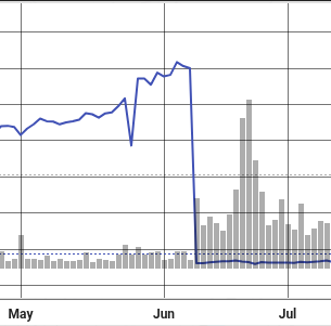
Even more subtly, corporate actions like stock splits can distort price series unless explicitly accounted for. For example, Nvidia’s 10-for-1 stock split on June 7, 2024, caused a sudden drop in share price purely due to adjustment — not market dynamics. Without proper normalization, strategies can misinterpret these events as volatility or crashes.
Even a simple idea like “find the most consistently traded stocks” turns out to depend on how you define consistency, and how well you understand the structure of your own dataset.
As this series of experiments suggests, there’s more to large-scale market data processing than meets the eye. It’s tempting to think of backtesting as a clean, deterministic pipeline — but in practice, the data fights back.
You’ll encounter missing or corrupted captures, incomplete trading days, symbols that appear midstream, and others that vanish without warning. Stocks get halted, merged, delisted, or IPO mid-cycle — all of which silently affect continuity, volume, and strategy logic.
Even more subtly, corporate actions like stock splits can distort price series unless explicitly accounted for. For example, Nvidia’s 10-for-1 stock split on June 7, 2024, caused a sudden drop in share price purely due to adjustment — not market dynamics. Without proper normalization, strategies can misinterpret these events as volatility or crashes.
Even a simple idea like “find the most consistently traded stocks” turns out to depend on how you define consistency, and how well you understand the structure of your own dataset.