Index

September 5, 2025
in finance, data-engineering, tools, quant
56 min read

I Analyzed 6TB of Raw Stock Market Data to Uncover the 30 Most Consistently Traded Stocks — Here’s What I Found

What if you could replay the last 9 years of market activity — every quote, every trade — and figure out which stocks have never left the party?

Stock Selection Last Friday, a quiet challenge came up in a conversation. Someone with a sharp mathematical mind and a preference for staying behind the scenes posed a deceptively simple question: "Which stocks have been traded the most, consistently, from 2016 to today?" That one question sent me down a 27-hour rabbit hole…

We had the data: 6TB of IEX tick captures spanning 2'187 PCAP files and over 22'119 unique symbols. We had the tools: an HDF5-backed firehose built for high-frequency analytics in pure C++23.

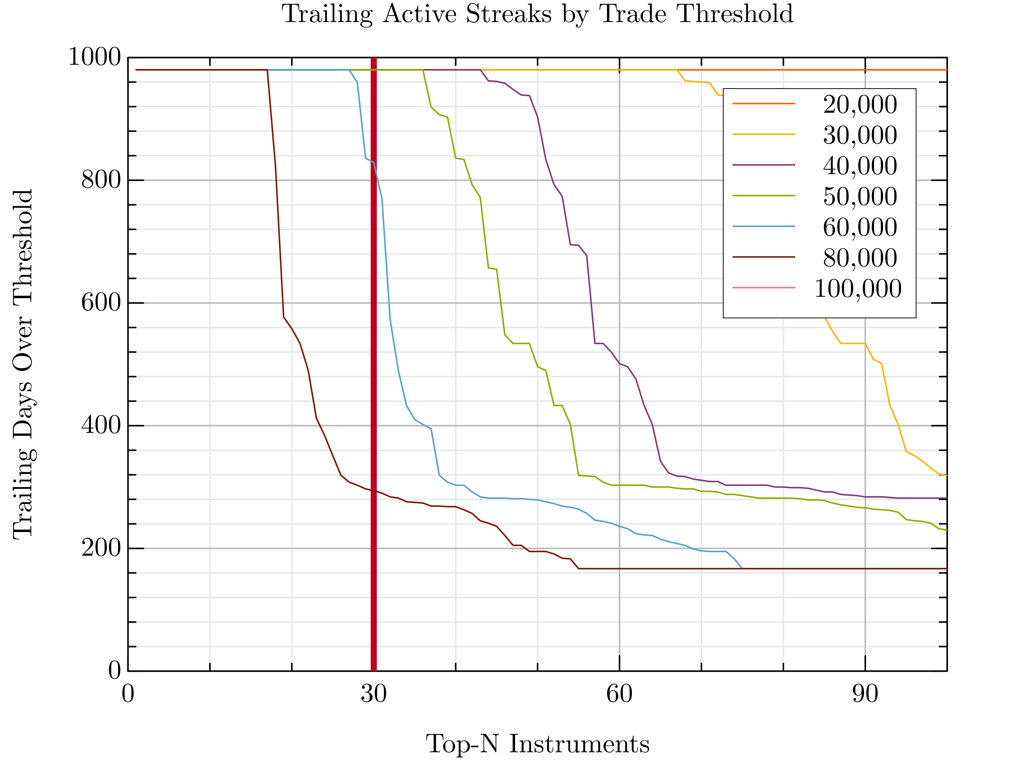
What followed was a misadventure in semantics. I first averaged trade counts across all dates — a rookie mistake. Turns out, averaging doesn’t guarantee consistency — some stocks burn bright for a while, then disappear. That oversight cost me half a day of CPU time and a good chunk of humility. The fix? A better idea: walk backwards from today and look for the longest uninterrupted streak of trading activity for each stock. Luckily, the 12 hours spent building the index weren’t wasted — that heavy lifting could be recycled for the new logic. Implementation time? 30 minutes. Execution time? 5 seconds. Victory? Priceless.

Here’s what we found.

Step 1 — Convert PCAPs into Stats with IEX2H5

Before we can rank stocks, we need summary statistics from the raw IEX market data feeds. That’s where iex2h5 comes in — a high-performance HDF5-based data converter purpose-built for handling PCAP dumps from IEX.

To extract stats only (and skip writing any tick data), we use the --command none mode. We'll name the output file something meaningful like statistics.h5, and pass in a file glob — the glorious Unix-era invention (from B at Bell Labs) — pointing to our compressed dataset, e.g. /lake/iex/tops/*.pcap.gz.

Of course, we’re all lazy, so let’s use the short forms -c, -o, and let iex2h5 do its thing:

steven@saturn:~/shared-tmp$ iex2h5 -c none -o statistics.h5 /lake/iex/tops/*.pcap.gz
[iex2h5] Converting 2194 files using backend: hdf5 — using 1 thread — © Varga Consulting, 2017–2025
[iex2h5] Visit https://vargaconsulting.github.io/iex2h5/ — Star it, Share it, Support Open Tools ⭐️
▫ 2016-12-13 14:30:00 21:00:00 ✓
▫ 2016-12-14 14:30:00 21:00:00 ✓
▫ 2016-12-15 17:31:52 21:00:00 ✓
[...]
▫ 2025-08-22 14:30:00 21:00:00 ✓
▫ 2025-08-25 14:30:00 21:00:00 ✓
▫ 2025-08-26 14:30:00 21:00:00 ✓
benchmark: 259159357724 events in 44087097ms  5.9 Mticks/s, 0.170000 µs/tick latency, 5758.33 GiB input converted into 733.97 MiB output
[iex2h5] Conversion complete — all files processed successfully 
[iex2h5] Market data © IEX — Investors Exchange. Attribution required. See https://iextrading.com

What you get is a compact HDF5 file containing:

/instruments → all unique stock symbols (22,119)
/trading_days → the full trading calendar (2,187 days)
/stats → per-symbol statistics across all days (e.g. trade volume, trade count, first/last seen)

On the performance side:

Raw storage throughput (ZFS): ~254 MB/s
End-to-end pipeline throughput: 5.76 TB of compressed PCAP input in 44,087 s → ~130 MB/s effective
Event rate: ~5.9 million ticks/sec sustained

From here you’re ready to rank, filter, and extract the top performers. The best part? A full 6 TB dataset was processed in ~12 hours — on a single desktop workstation, using a single-threaded execution model. No cluster, no parallel jobs.

These results form a solid baseline: the upcoming commercial version will extend the engine to a multi-process, multi-threaded execution model, scaling performance well beyond what a single core can deliver.

Step 2 — digest the statistics

Top-K Trade Streak Filter for Julia

using HDF5

base = homedir() * "/scratch"
input_file, output_file = base * "/index.h5", base * "/top30.h5"
cutoff_limit, lower_bound = 30, 50_000

fd = h5open(input_file, "r";  swmr=true)
function trailing_streak(x::AbstractVector{<:Real}, min::Real)
    count = 0
    for val in Iterators.reverse(x)
        val > min ? (count += 1) : break
    end
    return count
end

dates = String.(read(fd["/trading_days.txt"]))
instruments = String.(read(fd["/instruments.txt"]))

D, I = length(dates), length(instruments)
A = zeros(Float64, D, I)

for (day, date) in enumerate(dates)
    path = "/stats/$date/trade_size"
    if haskey(fd, path)
        count = vec(read(fd[path]))
        A[day, 1:length(count)] .= count
    end
end

# Step 2: Compute trailing streak length for each instrument
streak_lengths = [trailing_streak(A[:,i], lower_bound) for i in 1:I]

# Step 3: Rank instruments by streak length
order = sortperm(streak_lengths, rev=true)
selection = order[1:cutoff_limit]
h5_instruments = instruments[selection]
h5_trading_days = dates[end - minimum(streak_lengths[selection]) + 1:end]

# Step 4: Write result
h5open(output_file, "w") do fd
    write(fd, "/instruments.txt", h5_instruments)
    write(fd, "/trading_days.txt", h5_trading_days)
end

Top-K Trade Streak Filter for Python

#!/usr/bin/env python3
import numpy as np
import h5py
from pathlib import Path

base = Path.home() / "scratch"
input_file  = base / "index.h5"
output_file = base / "top30.h5"
cutoff_limit, lower_bound = 30, 50_000

fd = h5py.File(input_file, "r", swmr=True)
def trailing_streak(x: np.ndarray, min_val: float) -> int:
    cnt = 0
    for v in x[::-1]:
        if v > min_val:
            cnt += 1
        else:
            break
    return cnt

dates = fd["/trading_days.txt"][:].astype(str)
instruments = fd["/instruments.txt"][:].astype(str)

D, I = len(dates), len(instruments)
A = np.zeros((D, I), dtype=np.float64)

for day, date in enumerate(dates):
    path = f"/stats/{date}/trade_size"
    if path in fd:
        count = np.asarray(fd[path][()]).ravel()
        n = min(I, count.size)
        A[day, :n] = count[:n]

# Step 2: Compute trailing streak length for each instrument
streak_lengths = np.array([trailing_streak(A[:, i], lower_bound) for i in range(A.shape[1])])

# Step 3: Rank instruments by streak length
# DO NOT USE: it is not a stable sort, will diverge from julia implementation
#     order = np.argsort(-streak_lengths) 
order = np.lexsort((np.arange(len(streak_lengths)), -streak_lengths))

selection = order[:cutoff_limit]
h5_instruments = instruments[selection]
h5_trading_days = dates[-streak_lengths[selection].min():]

# Step 4: write result
str_dtype = h5py.string_dtype(encoding="utf-8")
with h5py.File(output_file, "w") as fd_out:
    fd_out.create_dataset("/instruments.txt", data=h5_instruments.astype(object), dtype=str_dtype)
    fd_out.create_dataset("/trading_days.txt", data=h5_trading_days.astype(object), dtype=str_dtype)

HDF5 data dump h5dump topk.h5

HDF5 "top30.h5" {
GROUP "/" {
   DATASET "instruments.txt" {
      DATATYPE  H5T_STRING {
         STRSIZE H5T_VARIABLE;
         STRPAD H5T_STR_NULLTERM;
         CSET H5T_CSET_UTF8;
         CTYPE H5T_C_S1;
      }
      DATASPACE  SIMPLE { ( 30 ) / ( 30 ) }
      DATA {
      (0): "EEM", "AAL", "HBAN", "TLT", "SQQQ", "CMCSA", "QQQ", "EWZ", "SPY",
      (9): "XLP", "CCL", "TSLA", "PLUG", "AMD", "NVDA", "XLF", "MU", "HYG",
      (18): "CSCO", "XLE", "IWM", "AAPL", "EFA", "TSM", "PCG", "INTC",
      (26): "VALE", "LQD", "FXI", "PBR"
      }
   }
   DATASET "trading_days.txt" {
      DATATYPE  H5T_STRING {
         STRSIZE H5T_VARIABLE;
         STRPAD H5T_STR_NULLTERM;
         CSET H5T_CSET_UTF8;
         CTYPE H5T_C_S1;
      }
      DATASPACE  SIMPLE { ( 980 ) / ( 980 ) }
      DATA {
      (0): "2021-09-13", "2021-09-14", "2021-09-15", "2021-09-16",
      (4): "2021-09-17", "2021-09-20", "2021-09-21", "2021-09-22",
      (972): "2025-08-15", "2025-08-18", "2025-08-19", "2025-08-20",
      (976): "2025-08-21", "2025-08-22", "2025-08-25", "2025-08-26"
      }
   }
}
}

Julia Plot

using Printf, Format
import GRUtils: oplot, plot, legend, xlabel, ylabel, title, savefig

colorscheme("solarized light")

thresholds = [20_000, 30_000, 40_000, 50_000, 60_000, 80_000, 100_000]
cutoff_limit,max = 30, 100

compute_streaks(A, min_val) = [trailing_streak(A[:, i], min_val) for i in 1:size(A, 2)]
sorted_streaks_per_threshold = Dict()
for t in thresholds
    streaks = compute_streaks(A, t)
    sorted_streaks_per_threshold[t] = sort(streaks, rev = true)[1:max]
end
plot([cutoff_limit, cutoff_limit], [0, 1000], "-r";
    linewidth=4, linestyle=:dash, xlim=(0, max), xticks=(10, 3), label=" 30")

for t in thresholds[1:end]
    oplot(1:length(sorted_streaks_per_threshold[t]),
          sorted_streaks_per_threshold[t]; label = format("{:>8}",format(t, commas=true)), lw = 2)
end

legend("")
xlabel("Top-N Instruments")
ylabel("Trailing Days Over Threshold")
title("Trailing Active Streaks by Trade Threshold")

Step 3 — Reprocess the Tick Data for the Top 30 Stocks

Now that we’ve identified the most consistently active stocks, it’s time to zoom in and reprocess just the relevant PCAP files. If you already have tick-level HDF5 output, you’re set. But if not, here's a neat trick: use good old Unix GLOB patterns to cherry-pick just the days you need — no need to touch all 6TB again.

For example, let’s reconstruct a trading window around September 2021:

iex2h5 -c irts -o top30.h5 /lake/iex/tops/TOPS-2021-09-1{3,4,5,6,7,8,9}.pcap.gz  # fractional start
iex2h5 -c irts -o top30.h5 /lake/iex/tops/TOPS-2021-09-{2,3}?.pcap.gz            # rest of the month

And then stitch together additional months or years:

iex2h5 -c irts -o top30.h5 /lake/iex/tops/TOPS-2021-1{0,1,2}-??.pcap.gz
iex2h5 -c irts -o top30.h5 /lake/iex/tops/TOPS-202{2,3,4,5}-??-??.pcap.gz

These globs target specific slices of the timeline while keeping file-level parallelism open for future optimization. And of course, you can always batch them via xargs.

Top-K Trade Streak Filter for Julia

using HDF5

base = homedir() * "/scratch"
input_file, output_file = base * "/index.h5", base * "/top30.h5"
cutoff_limit, lower_bound = 30, 50_000

fd = h5open(input_file, "r";  swmr=true)
function trailing_streak(x::AbstractVector{<:Real}, min::Real)
    count = 0
    for val in Iterators.reverse(x)
        val > min ? (count += 1) : break
    end
    return count
end

dates = String.(read(fd["/trading_days.txt"]))
instruments = String.(read(fd["/instruments.txt"]))

D, I = length(dates), length(instruments)
A = zeros(Float64, D, I)

for (day, date) in enumerate(dates)
    path = "/stats/$date/trade_size"
    if haskey(fd, path)
        count = vec(read(fd[path]))
        A[day, 1:length(count)] .= count
    end
end

# Step 2: Compute trailing streak length for each instrument
streak_lengths = [trailing_streak(A[:,i], lower_bound) for i in 1:I]

# Step 3: Rank instruments by streak length
order = sortperm(streak_lengths, rev=true)
selection = order[1:cutoff_limit]
h5_instruments = instruments[selection]
h5_trading_days = dates[end - minimum(streak_lengths[selection]) + 1:end]

# Step 4: Write result
h5open(output_file, "w") do fd
    write(fd, "/instruments.txt", h5_instruments)
    write(fd, "/trading_days.txt", h5_trading_days)
end

System Specs — Single Desktop Workstation (ZFS-backed)

This entire pipeline was executed on a single desktop workstation — no cluster, no GPU, no cloud — just efficient C++ and smart data layout:

CPU: Intel Core i7‑11700K @ 3.60 GHz (8 cores / 16 threads)
RAM: 64 GiB DDR4
Scratch Disk: 3.6 TB NVMe SSD (/mnt)
Main Archive: 15 TB ZFS pool (/lake), spanned 2× 8 TB HDDs
- Pool name: lake, Dataset: lake/stock, Compression: off (default), Recordsize: 128K (default), Deduplication: off
🐧 OS: Ubuntu 22.04 LTS

Read performance of ZFS based Lake 254MB/s sustained

steven@saturn:~$ sudo fio --name=zfs_seq_read_real --filename=/lake/fio-read-test.bin
    --rw=read --bs=1M --size=100G --numjobs=1 --ioengine=psync --direct=1 --group_reporting

zfs_seq_read_real: (g=0): rw=read, bs=(R) 1024KiB-1024KiB, (W) 1024KiB-1024KiB, (T) 1024KiB-1024KiB, ioengine=psync, iodepth=1
fio-3.28
Starting 1 process
zfs_seq_read_real: Laying out IO file (1 file / 102400MiB)
Jobs: 1 (f=1): [R(1)][100.0%][r=180MiB/s][r=180 IOPS][eta 00m:00s]
zfs_seq_read_real: (groupid=0, jobs=1): err= 0: pid=2897558: Sat Aug 30 16:40:16 2025
read: IOPS=242, BW=243MiB/s (254MB/s)(100GiB/422156msec)
    clat (usec): min=103, max=326105, avg=4118.30, stdev=8610.69
    lat (usec): min=104, max=326105, avg=4118.72, stdev=8610.67
    clat percentiles (usec):
    |  1.00th=[   208],  5.00th=[   229], 10.00th=[   277], 20.00th=[   824],
    | 30.00th=[   865], 40.00th=[   914], 50.00th=[  4146], 60.00th=[  4817],
    | 70.00th=[  5276], 80.00th=[  5800], 90.00th=[  6587], 95.00th=[  7767],
    | 99.00th=[ 33817], 99.50th=[ 61080], 99.90th=[102237], 99.95th=[139461],
    | 99.99th=[299893]
bw (  KiB/s): min=16384, max=395264, per=100.00%, avg=248505.24, stdev=59429.03, samples=843
iops        : min=   16, max=  386, avg=242.68, stdev=58.04, samples=843
lat (usec)   : 250=8.07%, 500=4.03%, 750=2.97%, 1000=28.82%
lat (msec)   : 2=1.16%, 4=3.06%, 10=49.77%, 20=0.87%, 50=0.56%
lat (msec)   : 100=0.60%, 250=0.08%, 500=0.03%
cpu          : usr=0.21%, sys=15.68%, ctx=58582, majf=0, minf=270
IO depths    : 1=100.0%, 2=0.0%, 4=0.0%, 8=0.0%, 16=0.0%, 32=0.0%, >=64=0.0%
    submit    : 0=0.0%, 4=100.0%, 8=0.0%, 16=0.0%, 32=0.0%, 64=0.0%, >=64=0.0%
    complete  : 0=0.0%, 4=100.0%, 8=0.0%, 16=0.0%, 32=0.0%, 64=0.0%, >=64=0.0%
    issued rwts: total=102400,0,0,0 short=0,0,0,0 dropped=0,0,0,0
    latency   : target=0, window=0, percentile=100.00%, depth=1

Run status group 0 (all jobs):
READ: bw=243MiB/s (254MB/s), 243MiB/s-243MiB/s (254MB/s-254MB/s), io=100GiB (107GB), run=422156-422156msec

Read performance of NVME scratch disk 4GB/s sustained

steven@saturn:~$ sudo fio --name=nvme_seq_read_real --filename=/home/steven/scratch/fio-read-test.bin
    --rw=read --bs=1M --size=100G --numjobs=1 --ioengine=psync --direct=1 --group_reporting
nvme_seq_read_real: (g=0): rw=read, bs=(R) 1024KiB-1024KiB, (W) 1024KiB-1024KiB, (T) 1024KiB-1024KiB, ioengine=psync, iodepth=1
fio-3.28
Starting 1 process
nvme_seq_read_real: Laying out IO file (1 file / 102400MiB)
Jobs: 1 (f=1): [R(1)][100.0%][r=3203MiB/s][r=3203 IOPS][eta 00m:00s]
nvme_seq_read_real: (groupid=0, jobs=1): err= 0: pid=3047825: Sat Aug 30 18:28:21 2025
read: IOPS=3847, BW=3848MiB/s (4035MB/s)(100GiB/26613msec)
    clat (usec): min=180, max=3871, avg=259.65, stdev=79.55
    lat (usec): min=180, max=3871, avg=259.68, stdev=79.56
    clat percentiles (usec):
    |  1.00th=[  198],  5.00th=[  200], 10.00th=[  202], 20.00th=[  202],
    | 30.00th=[  202], 40.00th=[  204], 50.00th=[  206], 60.00th=[  237],
    | 70.00th=[  310], 80.00th=[  318], 90.00th=[  371], 95.00th=[  400],
    | 99.00th=[  502], 99.50th=[  529], 99.90th=[  660], 99.95th=[  676],
    | 99.99th=[ 1106]
bw (  MiB/s): min= 2774, max= 4912, per=100.00%, avg=3852.79, stdev=798.23, samples=53
iops        : min= 2774, max= 4912, avg=3852.79, stdev=798.23, samples=53
lat (usec)   : 250=60.44%, 500=38.55%, 750=0.99%, 1000=0.01%
lat (msec)   : 2=0.01%, 4=0.01%
cpu          : usr=0.09%, sys=8.43%, ctx=102484, majf=0, minf=267
IO depths    : 1=100.0%, 2=0.0%, 4=0.0%, 8=0.0%, 16=0.0%, 32=0.0%, >=64=0.0%
    submit    : 0=0.0%, 4=100.0%, 8=0.0%, 16=0.0%, 32=0.0%, 64=0.0%, >=64=0.0%
    complete  : 0=0.0%, 4=100.0%, 8=0.0%, 16=0.0%, 32=0.0%, 64=0.0%, >=64=0.0%
    issued rwts: total=102400,0,0,0 short=0,0,0,0 dropped=0,0,0,0
    latency   : target=0, window=0, percentile=100.00%, depth=1

Run status group 0 (all jobs):
READ: bw=3848MiB/s (4035MB/s), 3848MiB/s-3848MiB/s (4035MB/s-4035MB/s), io=100GiB (107GB), run=26613-26613msec

Disk stats (read/write):
nvme0n1: ios=220152/422, merge=0/15, ticks=44398/64, in_queue=44537, util=99.70

Write performance of NVME scratch disk 2GB/s sustained

steven@saturn:~$ sudo fio --name=nvme_seq_write_real --filename=/home/steven/scratch/fio-write-test.bin
    --rw=write --bs=1M --size=100G --numjobs=1 --ioengine=psync --direct=1 --group_reporting

nvme_seq_write_real: (g=0): rw=write, bs=(R) 1024KiB-1024KiB, (W) 1024KiB-1024KiB, (T) 1024KiB-1024KiB, ioengine=psync, iodepth=1
fio-3.28
Starting 1 process
nvme_seq_write_real: Laying out IO file (1 file / 102400MiB)
Jobs: 1 (f=1): [W(1)][100.0%][w=1410MiB/s][w=1410 IOPS][eta 00m:00s]
nvme_seq_write_real: (groupid=0, jobs=1): err= 0: pid=3048070: Sat Aug 30 18:44:43 2025
write: IOPS=1989, BW=1990MiB/s (2087MB/s)(100GiB/51460msec); 0 zone resets
    clat (usec): min=211, max=232270, avg=462.02, stdev=3175.40
    lat (usec): min=232, max=232302, avg=502.00, stdev=3176.05
    clat percentiles (usec):
    |  1.00th=[   217],  5.00th=[   221], 10.00th=[   225], 20.00th=[   227],
    | 30.00th=[   229], 40.00th=[   233], 50.00th=[   241], 60.00th=[   281],
    | 70.00th=[   318], 80.00th=[   375], 90.00th=[   529], 95.00th=[   693],
    | 99.00th=[  1762], 99.50th=[  4883], 99.90th=[ 27132], 99.95th=[ 50070],
    | 99.99th=[149947]
bw (  MiB/s): min=  534, max= 3574, per=100.00%, avg=1997.23, stdev=784.43, samples=102
iops        : min=  534, max= 3574, avg=1997.15, stdev=784.48, samples=102
lat (usec)   : 250=52.21%, 500=36.83%, 750=6.89%, 1000=1.85%
lat (msec)   : 2=1.34%, 4=0.31%, 10=0.22%, 20=0.14%, 50=0.17%
lat (msec)   : 100=0.02%, 250=0.03%
cpu          : usr=8.02%, sys=23.04%, ctx=102593, majf=0, minf=14
IO depths    : 1=100.0%, 2=0.0%, 4=0.0%, 8=0.0%, 16=0.0%, 32=0.0%, >=64=0.0%
    submit    : 0=0.0%, 4=100.0%, 8=0.0%, 16=0.0%, 32=0.0%, 64=0.0%, >=64=0.0%
    complete  : 0=0.0%, 4=100.0%, 8=0.0%, 16=0.0%, 32=0.0%, 64=0.0%, >=64=0.0%
    issued rwts: total=0,102400,0,0 short=0,0,0,0 dropped=0,0,0,0
    latency   : target=0, window=0, percentile=100.00%, depth=1

Run status group 0 (all jobs):
WRITE: bw=1990MiB/s (2087MB/s), 1990MiB/s-1990MiB/s (2087MB/s-2087MB/s), io=100GiB (107GB), run=51460-51460msec

Disk stats (read/write):
nvme0n1: ios=6052/319248, merge=0/35, ticks=4761/121381, in_queue=138161, util=95.95%

Lessons from the Data Trenches

Stock Selection As this series of experiments suggests, there’s more to large-scale market data processing than meets the eye. It’s tempting to think of backtesting as a clean, deterministic pipeline — but in practice, the data fights back. You’ll encounter missing or corrupted captures, incomplete trading days, symbols that appear midstream, and others that vanish without warning. Stocks get halted, merged, delisted, or IPO mid-cycle — all of which silently affect continuity, volume, and strategy logic. Even more subtly, corporate actions like stock splits can distort price series unless explicitly accounted for. For example, Nvidia’s 10-for-1 stock split on June 7, 2024, caused a sudden drop in share price purely due to adjustment — not market dynamics. Without proper normalization, strategies can misinterpret these events as volatility or crashes. Even a simple idea like “find the most consistently traded stocks” turns out to depend on how you define consistency, and how well you understand the structure of your own dataset.

August 23, 2025
in encoding, hdf5, c++
5 min read

Radix64 Encoding: Order-Preserving Strings in 64 Bits

Problem: Compact, Order-Preserving Identifiers for Short Symbols

In domains like high-frequency trading, structured storage, or financial indexing, identifiers such as stock symbols (e.g., "AAPL", "GOOG", "TSLA") are:

Short — typically ≤ 8 characters
Drawn from a small alphabet — ~32 to 40 printable characters
Compared lexicographically — e.g., "ABC" < "XYZ" must hold

These structural constraints can be exploited to encode each symbol into a compact, fixed-width binary key while preserving their natural sort order.

Specifically, such systems often need:

Lexicographic ordering — to maintain sorted maps, symbol trees, or search indices
Fixed-size keys — for CPU- and cache-friendly performance
Support for variable-length symbols — without breaking ordering
Ability to pack extra metadata — like 16-bit contract IDs or timestamps

But typical representations fall short:

std::string / char[] are variable-length and inefficient as keys
strcmp is slow, branching, and non-SIMD friendly
Standard Base64 isn't order-preserving
Hashes destroy ordering and increase collision risk

➤ Radix64 encoding solves this by leveraging the symbol structure — short, constrained, ordered strings — to pack lex-order-preserving representations into just 64 bits.

Solution: Order-Preserving Radix64 Encoding

Radix64 solves this by:

Encoding up to 8 characters as a 48-bit big-endian base-64 integer
Padding shorter strings with the lowest code to preserve prefix order
Optionally combining a 16-bit integer (e.g., contract ID) in the LSBs
Making unsigned integer comparison exactly match lexicographic order

So you can now represent things like:

"AAPL"    → 48-bit radix64 prefix
contract  → 16-bit index
key       → 64-bit sortable, compact ID

Used as keys in:

Fast symbol lookup tables
Order books and trading systems
Encoded identifiers for datasets or HDF5 groups
Key-value stores, B-trees, or radix trees

Read the full radix64 guide

May 12, 2025
in blockchain, cryptography, julia
8 min read

From Curve to Signature: A Hands-on Guide to ECDSA

ECDSA operates on elliptic curve groups over finite fields.
In the most common form, the curve is defined by the Weierstrass equation:\(E(\mathbb{F}_p):\; y^2 \equiv x^3 + ax + b \pmod p,\) where \(a, b\) are curve parameters and \(p\) is a prime defining the field \(\mathbb{F}_p\). In production systems, the curve is fixed by cryptographers — for example, secp256k1 in Ethereum — but nothing prevents you from experimenting with your own, especially for learning, prototyping, or testing with small primes.

Generate a toy Weierstrass curve

This example searches for a curve over primes \(\pi \in (97,103)\), with parameters \(a \in (10,15)\), \(b \in (2,7)\). It selects the first candidate that is non-singular, whose group of points has prime order, and that admits a generator spanning the group.

using TinyCrypto

curve = Weierstrass(97:103, 10:15, 2:7)
Weierstrass{𝔽₉₇}: y² = x³ + 10x + 3 | 𝔾(0,10), q = 101, h = 1, #E = 101

Here, \(q\) is the order of the generator \(\mathbb{G} (0𝔽₉₇,10𝔽₉₇)\), \(h\) the cofactor, and \(\#E = q \cdot h\) the total number of points on the curve.

Sign a Message (ECDSA)

priv, pub = genkey(curve)             # Generate private/public key pair
msg = "hello ethereum"                # The message to sign
signature = sign(curve, priv, msg)    # → (r, s, v)

The result is a NamedTuple:

(r = ..., s = ..., v = ...)

Here, \((r,s)\) are the ECDSA signature scalars, and \(v\) is the recovery identifier — letting you reconstruct the signer’s public key from the signature and message alone. This is exactly how Ethereum transactions prove authenticity without revealing the private key.

Verify the Signature

is_valid = verify(curve, pub, signature, msg)
@assert is_valid

Verification checks that the signature \((r,s)\) was produced with the private key corresponding to the public key pub, on the exact message msg. If the check passes, you know the message is authentic and unaltered — the essence of digital signatures in action.

Recover the Public Key (like Ethereum)

recovered = ecrecover(curve, msg, signature)
@assert pub == recovered

ECDSA with recovery adds a small extra bit \(v\) to the signature, making it possible to reconstruct the signer’s public key directly from (msg, signature). This is how Ethereum avoids shipping full public keys inside every transaction: the network can derive them on the fly, saving space while still proving who signed what.

Summary

TinyCrypto.jl makes it easy to:

Define toy elliptic curves over small prime fields
Generate key pairs and sign messages with ECDSA
Verify signatures to ensure authenticity and integrity
Recover public keys from signatures (à la Ethereum)

Perfect for learning, prototyping, or experimenting with elliptic curve cryptography — without the overhead of production-grade libraries.

🔗 Source code on GitHub

May 17, 2023
in hdf5, c++
6 min read

Why Your HDF5 Dataset Can't Extend—and the H5CPP Way

Rudresh shared that attempts to extend a dataset were failing with crashes or no effect—despite calling .extend(...) or H5Dextend(). Their code was creating a 2D dataset of variable‑length strings, but had not enabled chunking or specified unlimited max dimensions, leaving them stuck.

The Insight

If you don’t create a dataset with chunked layout and max dimensions set to unlimited (H5S_UNLIMITED), HDF5 creates it with contiguous storage and a fixed size that cannot be extended later. That's the crux: without chunking and unlimited dims, calling .extend will fail or crash.

A Possible H5CPP Solution

Here’s how you can cleanly create an extendible dataset and append to it—using H5CPP:

#include <h5cpp/all>

int main() {
  // Create a new file and an extendible dataset of scalar values
  h5::fd_t fd = h5::create("example.h5", H5F_ACC_TRUNC);

  // Create a packet-table (extendible) dataset of scalars
  h5::pt_t pt = h5::create<size_t>(
    fd, 
    "stream of scalars", 
    h5::max_dims{H5S_UNLIMITED}
  );

  // Append values dynamically
  for (auto value : {1, 2, 3, 4, 5}) {
    h5::append(pt, value);
  }
}

For a frame‑by‑frame stream (e.g., matrices or images):

#include <h5cpp/all>
#include <armadillo>

int main() {
  h5::fd_t fd = h5::create("example.h5", H5F_ACC_TRUNC);
  size_t nrows = 2, ncols = 5, nframes = 3;

  auto pt = h5::create<double>(
    fd,
    "stream of matrices",
    h5::max_dims{H5S_UNLIMITED, nrows, ncols},
    h5::chunk{1, nrows, ncols}
  );

  arma::mat M(nrows, ncols);
  for (int i = 0; i < nframes; ++i) {
    h5::append(pt, M);
  }
}

Why This Works

Aspect	H5CPP Approach
Extendible storage	`h5::max_dims{H5S_UNLIMITED}`
Chunked layout setup	Automatic via `h5::chunk{...}`
Appending data	One-liners with `h5::append(...)`
Clean C++ modern API	Templates, RAII, zero boilerplate

TLDR

If your HDF5 dataset “can’t extend,” the culprit is almost always that it's not chunked with unlimited dimensions. Fix that creation pattern—chunking is mandatory. With H5CPP, appending becomes elegant and idiomatic:

Create: h5::create with unlimited dims
Append: h5::append(...) in plain C++ style

Let me know if you'd like this turned into a tutorial or compared to the raw HDF5 C++ API equivalent.

April 17, 2023
in hdf5, c++
6 min read

Optimizing Reads of Very-Wide Compound HDF5 Types

The User’s Problem (Matt, Apr 2023)

Matt is struggling with reading HDF5 datasets comprised of extremely wide compound types (think up to ~460 fields):

Data is stored as an Nx1 array of compound structs with hundreds of fields, compressed with gzip.
Reads dominate runtime (90%)—mostly in Python/h5py.
In practice, they need all rows, but only a small subset of fields. Yet, reading a single field one at a time is slow; full-row reads are even slower.
Splitting each field into its own dataset killed write performance; the current design isn’t cutting it.

My Take: Swap Width for Depth With Smart Packing

Here’s how I’d rethink the layout from an HDF5/H5CPP standpoint:

1. Chunking + Field Grouping

Pack related fields together into chunked arrays, based on how they’re queried, not just what’s easiest to write.

Define blocks (chunks) where each contains a subset of fields that you often read together.
That way, each read aligns with your real access pattern, boosting I/O efficiency.
Yes, some fields may be stored twice in different chunks—but that’s a conscious space-for-speed trade-off.

2. Optimize Based on Queries

Design your dataset structure backward—from the query patterns, not upstream modeling considerations. Pre-encode access patterns in your layout.

Summary Table

Strategy	Pros	Trade-Offs
Wide compound structs	Simple to write	Slow for selective reads
Per-field datasets	Very selective reads	Sluggish writes, many datasets
Chunked field grouping (recommended)	Fast reads for grouped fields, aligned I/O	Slight redundancy, more planning

TL;DR

Reading “all rows but a few fields” from hundreds-wide compound datasets can crush performance, especially in Python.

The fix? Restructure your HDF5 layout to align with real query behavior—use chunked blocks that contain all frequently accessed fields together. H5CPP supports this cleanly with a modern template-based API.

March 28, 2023
in hdf5, c++
10 min read

HDF5 Write Speeds: Matching Underlying Raw I/O

The Question (OP Concern)

A user observed that writing huge blocks (≥10 GB) with HDF5 was noticeably slower than equivalent raw writes. Understandably—they're comparing structured I/O to unadorned write() calls. The question: is this performance gap unavoidable, or can HDF5 be tuned to catch up?

What I Found (Steven Varga, Mar 28, 2023)

Here’s what I discovered—and benchmarked—on my Lenovo X1 running a recent Linux setup:

Running a cross‑product H5CPP benchmark, I consistently hit about 70–95% of the raw file system’s throughput when writing large blocks—clear evidence HDF5 is not inherently slow at scale.
With tiny or fragmented writes, overhead becomes a bigger issue—as Gerd already pointed out, direct chunk I/O is the key to performance there. Rebuild your own packer or write path around full chunks.
Or, if you want simplicity with speed, use H5CPP’s h5::append(). It streamlines buffered I/O, chunk alignment, and high throughput without manual hackery.

Here’s a snippet from my test run:

steven@io:~/projects/h5bench/examples/capi$ make
g++ -I/usr/local/include -I/usr/include -I../../include -o capi-test.o   -std=c++17 -Wno-attributes -c capi-test.cpp
g++ capi-test.o -lhdf5  -lz -ldl -lm -o capi-test
taskset 0x1 ./capi-test
[name                                              ][total events][Mi events/s] [ms runtime / stddev] [    MiB/s / stddev ]
fixed length string CAPI                                    10000     625.0000         0.02     0.000   24461.70     256.9
fixed length string CAPI                                   100000     122.7898         0.81     0.038    4917.70     213.3
fixed length string CAPI                                  1000000      80.4531        12.43     0.217    3218.60      56.6
fixed length string CAPI                                 10000000      79.7568       125.38     0.140    3189.80       3.6
rm capi-test.o

int main(int argc, const char **argv){
  size_t max_size = *std::max_element(record_size.begin(), record_size.end());

  h5::fd_t fd = h5::create("h5cpp.h5", H5F_ACC_TRUNC);
  auto strings = h5::utils::get_test_data<std::string>(max_size, 10, sizeof(fl_string_t));
    std::vector<char[sizeof(fl_string_t)]> data(strings.size());
        for (size_t i = 0; i < data.size(); i++)
            strncpy(data[i], strings[i].data(), sizeof(fl_string_t));

  // set the transfer size for each batch
  std::vector<size_t> transfer_size;
  for (auto i : record_size)
      transfer_size.push_back(i * sizeof(fl_string_t));

  //use H5CPP  modify VL type to fixed length
  h5::dt_t<fl_string_t> dt{H5Tcreate(H5T_STRING, sizeof(fl_string_t))};
  H5Tset_cset(dt, H5T_CSET_UTF8);

  std::vector<h5::ds_t> ds;
  // create separate dataset for each batch
  for(auto size: record_size) ds.push_back(
    h5::create<fl_string_t>(fd, fmt::format("fixe length string CAPI-{:010d}", size), 
    chunk_size, h5::current_dims{size}, dt));

  // EXPERIMENT: arguments, including lambda function may be passed in arbitrary order
  bh::throughput(
    bh::name{"fixed length string CAPI"}, record_size, warmup, sample,
    [&](size_t idx, size_t size_) -> double {
        hsize_t size = size_;
        // memory space
        h5::sp_t mem_space{H5Screate_simple(1, &size, nullptr )};
        H5Sselect_all(mem_space);
        // file space
        h5::sp_t file_space{H5Dget_space(ds[idx])};
        H5Sselect_all(file_space);
        // IO call
        H5Dwrite( ds[idx], dt, mem_space, file_space, H5P_DEFAULT, data.data());
        return transfer_size[idx];
    });
}

So, large writes are nearly as fast as raw file writes. The performance dip is most pronounced with smaller payloads.

What This Means In Practice

Write Size	HDF5 Performance	Takeaway
Large contiguous	~70–95% of raw I/O	HDF5 is performant at scale
Small fragments	Lower efficiency	Use chunk-based buffering
Need simplicity + speed	Use `h5::append()`	Combines clarity and performance

TL;DR

HDF5 is fast—large-block writes approach raw I/O speeds.
Inefficiency creeps in with tiny or non-aligned writes.
Solution? Direct chunk I/O or use H5CPP’s h5::append() for elegant, high-throughput data streaming.

March 24, 2023
in hdf5, c++
6 min read

Why Writing HDF5 Chunks Piece-by-Piece Actually Fails

The Question (March 20, 2023)

The OP wanted to bypass copying and buffering in memory by writing HDF5 chunks in parts—i.e., building them incrementally. They’d heard of using H5Dget_chunk_info plus pwrite() to patch up chunk contents manually, especially in uncompressed scenarios.

My Response (March 24, 2023)

Let me clarify the constraints first: a chunk is an indivisible IO unit in HDF5. It is processed as a single atomic job—particularly vital if filters or compression are applied. That’s baked into the library semantics and reflects how most storage and memory subsystems work.

Here’s how you'd typically handle data in that model:

Chunk-based pipeline (e.g., with block ciphers): 1. pread(fd, data, full_chunk_size, offset) 2. Repeat until the entire chunk is loaded (must be whole) 3. Apply filters/pipelines to the chunk 4. Write or process…

Given this model, partial chunk writes simply don’t make sense—and won’t be accepted by HDF5’s filter chain integrity checks.

What You Should Do Instead

Read the entire chunk, decode it, process your changes, then write the full chunk back. It’s the only correct way.
If naive, direct chunk operations hit 90%+ of NVMe bandwidth in benchmarks, you're already in a sweet spot—focus on optimizing higher-level logic.
H5CPP’s h5::packet_table elevates this approach: it abstracts buffer management and chunk alignment, so you can safely accumulate data from multiple sources and efficiently flush complete chunks.

TL;DR

Chunk Behavior	You Must Do	H5CPP Helps With
Filter/compression atomicity	Always read and write full chunk	`h5::packet_table` handles pre-buffering and alignment
Fragment writes	Not supported	Use full chunk replacement workflow
Performance on NVMe	Good if chunked properly	Fine-tuned by `h5::append()` internals

Let me know if you'd like a code breakdown of h5::packet_table or a deep dive on how to handle chunk durability and concurrency in a streaming pipeline.

March 20, 2023
in hdf5, c++
7 min read

Writing Direct HDF5 Chunks Piece-by-Piece with H5CPP

The Use Case (OP Context)

You’re working in a system that ingests data from multiple queues or streams, and you want to aggregate and flush them into HDF5 chunks incrementally. Essentially you need fine control: pack incoming data, apply filters, and write out only full chunks—or directly stream partial ones—without sacrificing alignment or performance.

My H5CPP-Based Guidance

See h5cpp::packet_table on GitHub—it's designed for chunked, appendable writes. It features a chunk-packing mechanism and a filter-chain you can adapt for your needs. I even slipped in an alignment bug (huge respect to Bin Dong at Berkeley for spotting it)—you’ll only run into it if your chunks aren’t properly aligned.

You should be able to modify h5::append so that it aggregates data from different queues and flushes when chunks are full. For inspiration, check the repository example that demonstrates how to use lock‑free queues and ZeroMQ with both C++ and Fortran.

H5CPP Pattern at Work

Here’s the essence of how you can architect this:

Use a packet table (extendable dataset) to buffer incoming records.
Customize h5::append():
Buffer data from various queues
Apply filters or transformations as needed
Write when a full chunk forms or at flush points
Ensure chunk alignment consistently to avoid edge-case bugs.
Support multi-threaded or multi-logic producers via lock-free queues or messaging systems like ZeroMQ.
Check the example repo for C++ and Fortran operators integrating queues + chunk flush logic.

Why This Matters

Requirement	H5CPP Approach
Incremental append (partial/final chunks)	Override or wrap `h5::append()`
Safe aggregation from multiple streams	Use lock-free queues, ZeroMQ patterns
High throughput + minimal latency	Chunk packing with filter chain support
Alignment-sensitive writes	Align chunks to avoid subtle bugs
Cross-language producer support (e.g. Fortran)	Example-driven integration from H5CPP repo

TL;DR

To write HDF5 chunks piece-by-piece in a high-performance, multi-source pipeline:

Start with the H5CPP packet-table abstraction.
Adapt h5::append() to batch and flush chunks from multiple inputs.
Keep chunk boundaries aligned—watch out for that subtle alignment bug!
Leverage lock-free queues or messaging for producer side decoupling.
Check the H5CPP repo examples for inspiration, even in multi-language setups.

Let me know if you'd like to walk through a C++ code snippet or a multi-threaded producer example using this pattern.

— Steven Varga

March 2, 2023
in hdf5, c++
6 min read

Extendable Datasets in HDF5—Simplified with H5CPP

The OP’s Context

The user wanted to create an HDF5 dataset that can grow over time—think event streams or log records—and do so with a clean C++ interface. Writing their own solution was on the table, but they were seeking something performant and maintainable.

H5CPP to the Rescue (Steven Varga, Mar 2 2023)

“Probably you want to roll your own, which is a good thing—but in case you're looking for a performant solution:”

#include <h5cpp/core>
#include "generated.h"  // your record type mapping
#include <h5cpp/io>
int main(){
  auto fd = h5::create("test.h5", H5F_ACC_TRUNC);
  { // Create an extendable dataset with your POD struct
    auto ds = h5::create<sn::record_t>(
      fd, "/path/dataset", h5::max_dims{H5S_UNLIMITED});
    // Assign vector-of-strings attribute
    ds["attribute"] = {"first","second","...","last"};
    // Convert dataset to packet-table and append records
    auto pt = ds;
    for (int i = 0; i < 3; ++i) {
      h5::append(pt, sn::record_t{
        1.0 * i, 2.0 *i,
        {1,2,3,4,5}, {11,12,13,14,15}
      });
    }
  }
  { // Read back the dataset
    auto ds = h5::open(fd, "/path/dataset");
    auto attribute = h5::aread<std::vector<std::string>>(ds, "attribute");
    std::cout << attribute << std::endl;
    // Dump data
    for (auto rec : h5::read<std::vector<sn::record_t>>(ds, "/path/dataset"))
      std::cerr << rec.A << " ";
    std::cerr << std::endl;
  }
}

Why This Works So Nicely

Feature	Benefit
`H5S_UNLIMITED` max dims	Enables true extendible dataset
`sn::record_t` POD mapping	Compact and expressive schema definitions
`h5::append(...)` API	Simple, zero-boilerplate appends
Packet-table behind the scenes	Efficient I/O under the hood
Vector attribute support	Seamless metadata attachment and retrieval

TL;DR

Creating appendable, extendable datasets in C++ is no longer boilerplate-heavy. H5CPP gives you:

C++ templates for structure mapping
Clean append logic with h5::append()
Flexible storage with unlimited dataspace
Convenient metadata via attributes

June 29, 2022
in hdf5, c++
6 min read

sudo apt-get install libzmq3-dev
````

#### Python:

```bash
python3 -m pip install pyzmq

Fortran ZMQ bindings:

Install fzmq:

git clone https://github.com/richsnyder/fzmq && cd fzmq
mkdir build && cd build
cmake -DBUILD_DOCS=OFF ../
sudo make install

🛰️ Sender: Python

#!/usr/bin/python3
import zmq

ctx = zmq.Context()
sock = ctx.socket(zmq.PUSH)
sock.connect("tcp://localhost:5555")

for x in range(100):
    sock.send(x.to_bytes(8, 'little'))

Highlights:

Sends 8-byte integers in little-endian format
Easy for testing other receivers

🛰️ Sender: C++

#include <zmq.h>
#include <cstdint>
#include <cstring>

int main() {
    void* ctx = zmq_ctx_new();
    void* sock = zmq_socket(ctx, ZMQ_PUSH);
    zmq_connect(sock, "tcp://localhost:5555");

    for(uint64_t x = 0; x < 100; ++x)
        zmq_send(sock, &x, sizeof(x), 0);

    zmq_close(sock);
    zmq_ctx_term(ctx);
}

Highlights:

Sends raw uint64_t values (8 bytes)
Matches Python format

🛰️ Sender: Fortran

program send
  use fzmq
  implicit none

  type(zmq_context) :: context
  type(zmq_socket)  :: sock
  integer(kind=8)   :: x
  integer           :: rc

  context = zmq_ctx_new()
  sock = zmq_socket(context, ZMQ_PUSH)
  call zmq_connect(sock, "tcp://localhost:5555")

  do x = 0, 99
    call zmq_send(sock, x, 8, 0)
  end do

  call zmq_close(sock)
  call zmq_ctx_term(context)
end program send

Highlights:

Uses fzmq bindings
Sends binary 64-bit integers

🎯 Receiver: C++

#include <zmq.h>
#include <cstdint>
#include <cstdio>

int main() {
    void* ctx = zmq_ctx_new();
    void* sock = zmq_socket(ctx, ZMQ_PULL);
    zmq_bind(sock, "tcp://*:5555");

    for(uint64_t x; true;) {
        zmq_recv(sock, &x, sizeof(x), 0);
        printf("recv: %lu\n", x);
    }

    zmq_close(sock);
    zmq_ctx_term(ctx);
}

Highlights:

Pulls 64-bit integers from any connected sender
No language-specific deserialization required

✅ Summary

ZeroMQ’s PUSH/PULL pattern makes multi-language IPC a breeze.

Role	Language	Notes
Sender	Python	Uses `pyzmq`, clean syntax
Sender	C++	Raw `zmq_send` of binary integers
Sender	Fortran	Uses `fzmq` bindings
Receiver	C++	Prints values from all senders

Run the receiver first, then launch any combination of senders. Messages will stream in regardless of language. No serialization frameworks, no boilerplate.